Let's Learn
1. What is Data Structure?
2. Classification & Commonly Used Data Structures
- Linear Data Structures
Arrays,
Stack,
Queue,
Linked List.
- Non-Linear Data Structures
Binary Tree,
Heap,
Graphs,
Hash Table.
WHAT IS DATA STRUCTURE
Data Structure refers to the way in which digital data units are structured in an organized form. Data structures are broadly classified into two.
1. Linear Data Structures - Here data elements are stored/retrieved sequentially.
Examples: Arrays, Stack, Queue, Linked List
2. Non-Linear Data Structures - Here data elements are not stored/retrieved sequentially.
Examples: Binary Tree, Heap, Graphs, Hash Table
Data Structures are used for the efficient storage and reliable management of data. Any professional programmer must have a fair understanding of what Data Structures are. Software architects comfortably handle data structures during system design stage of complex applications.
Linear Data Structure : ARRAYS
Array is the collection of fixed consecutive memory units that store same data-type values. It is identified by a common name and individual memory units are referred by their index number.
In this figure, int a[5] is an array of integer elements, collectively named a. These elements are numbered from 0 to 4 since in arrays, the first index always starts from 0.
It can store 5 integer values at contiguous memory locations named (or indexed) as a[0], a[1], a[2], a[3] and a[4]. Values within the array elements can be traversed by referring to the array indexes.
A new element cannot be added to an array and existing element cannot be deleted from the array as array elements are static (fixed) in size. However, values within array elements can be replaced.
TYPES OF ARRAYS
More commonly used arrays are: One-Dimensional arrays and Two-Dimensional arrays
One-Dimensional Array
The one-dimensional array can be a row with multiple columns:
or a column with multiple rows:
Two-Dimensional Arrays
The two-dimensional array holds data values of similar data-type in multiple rows, and multiple columns.
Each elements in a multidimensional array is referred by its row-column index. In the given figure, ‘a’ is an integer array with 3 rows and 4 columns.
The first element of this array is the top left corner referred as a[0][0]. Traversing through this array, the last element is at bottom right corner marked by a[2][3].
Linear Data Structure : STACK
A stack of plates is a relatable example, where new plates are placed at the top, and most recent plate will be the first to be removed.
Hence in a Stack, the data elements are inserted or deleted from the top as in the Last In First Out (LIFO) order. The stack operation is applied for processing recursive function calls.
Adding elements to a stack is termed as push. Deleting elements from a stack is termed pop.
Linear Data Structure : QUEUE
The queue in a ticket counter is an example where the first person entering a queue is the first to exit.
Queue follows the First In First Out (FIFO) order where data elements are added from rear-end and deleted from the top. It finds application in streaming operations, printer scheduling tasks, multi-threading etc.
Adding elements via the rear of a queue is termed enqueue, and deleting elements from front of a queue is termed dequeue.
Linear Data Structure : Linked List
Linked lists are a distributed collection of nodes (memory units with accessible memory address) that not only stores data values but also helps traverse to the next, or to previous data-nodes.
Each node carries within it a data-value, and a pointer to memory address of “next” node, and also the pointer to address of “previous” node.
The start location is a pointer that will store address of first data-node, while the end pointer will store address of the last data-node.
What we learned here is a doubly linked list where data is accessed both forwards & backwards in a sequential manner (not random access).
There are linked lists that traverse either in forward direction or those that traverse in a backward direction. Such linked lists are termed as the singly linked list.
Non-Linear Data Structure : Binary Tree
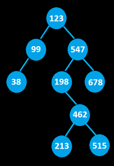
The binary tree is one of the most commonly used tree data structures where data is organized and linked as nodes in a hierarchical (ordered) or sorted manner.
A binary search tree starts with the root node and spreads its branches downwards. Each node has 2 child nodes where left node stores the next data-value if it is less than the parent node, and right node stores data-value if it is greater than the parent node.
As nodes increase, it takes the form of an inverted tree with the root at top, followed by it’s branches, then the child nodes (or the siblings), and finally the leaves (nodes with no child). Hence its termed the binary tree.
A binary tree is implemented by linked lists where incessant search, insertion, or deletion of data-nodes are efficiently executed at a rapid pace.
Non-Linear Data Structure : Heap
The Heap data-structure is a binary tree where value of parent node is compared to that of its child nodes and is then arranged either as maximum sequence (max-heap) or minimum sequence (min-heap).
In max-heap the root-node will carry maximum value of the heap, and value in each parent will be greater than or equal to those of its children.
In min-heap the root-node will carry minimum value of the heap, and value in each parent will be lesser than or equal to those of its children.
The heap is a complete binary tree, but partially ordered, that is used in heapsort algorithm and to execute priority queues.
Non-Linear Data Structure : Graphs
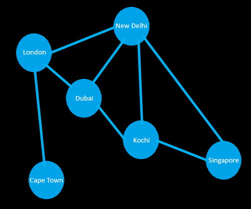
The Graph comprise of data-nodes (vertices) that can have multiple connections (edges) forming cohesive data clusters. The number of vertices refers to order of a graph and the number of edges corresponds to size of a graph. Graphs can be Undirected, or Directed, or Weighted.
Undirected Graph
Directed Graph
Weighted Graph
Graphs help model nodes with modern day real-world networks where connections are managed by clustering algorithms that feed on data from distributed & neural networks. Hence it finds wide applications;
in Market Segmentation (grouping of huge customer data for different market segments),
in Social Network Analysis (eg. predicting friends list),
in Server Farm Resources (where huge data is split & distributed for speed & safety)
... and so on.
Non-Linear Data Structure : Hash Table
Hash tables (hash maps) are basically unordered lists that are used to store information about key-value pairs. It comprises of 2 major parts:
- a Key (reference code) which is unique,
- a Value (data),
where every key is mapped (refers) to a corresponding data value.
When we need to speed up search operations for voluminous data, we opt to use hash tables, because the hash-key can directly point to a hash-value.
Hash tables are basically implemented in arrays and or lists.
Functioning of a Hash Map
The keys used in hash maps will undergo hashing technique to generate indexes of integer values. The key is then stored in these “array or list” indexes for quick storage or retrieval.
In hashing technique, the hash function uses some sort of a formula to convert the key into an index. The index corresponding to a key is then stored in the hash table.
Lets consider a hash table. its just a file, with a large volume of key-value pairs. Searching for the last data here would mean traversing each record of the file, & searching for the required data corresponding to a given specified key. In the hash table, we create an index for each key-value pair, & find ways to quickly point to specific indexes, so that data can be retrieved significantly fast. The so called "index" is created by a hash function, into which the KEY is passed. The hash function we are going to have here uses a formula (in fact any formula we can think of under the sun!!), where it finds modulo of KEY value & the array, or list size.
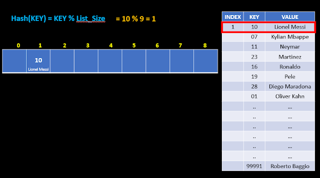
Hash(KEY) = KEY % List_Size
Here array size will be 9, as our list has 9 elements (see the image just before the last one).
Lets now find index for the first row in the table. The key is 10. So 10 mode 9 would mean, divide 10 by 9, & get the remainder. Its 1. Hence index for the first row is recorded as 1. & hence, the key 10, of our first row, is stored in element 1 of the list, along with its data-value "Lionel Messi".
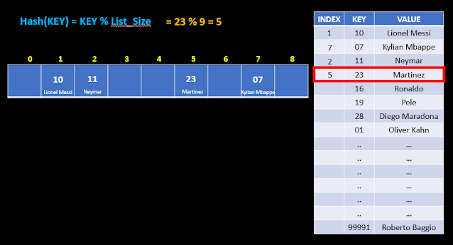
For the next row, its 7 mode 9, & the answer is 7. So key 07 along with its data-value "Kylian Mbappe", is stored at index 7.
In the next row its 11 mode 9, or 2. & so 11, or Neymar, is stored at index 2 of list.
The next index is 23 mode 9, or 5. So 23 & Martinez are stored at index 5 of list.
Now comes the interesting turn.
In the next row, index would be 16 mode 9, or 7. Here, there is a repetition of the index. We already have an index 7 for the key 07 & data-value Mbappe. This logjam is termed collision, & the resolution is to implement what is called "bucket hashing". It means to simply create a storage bucket for the index where the logjam has occurred. The bucket helps to pile up multiple key-value pairs in common indexes. So here, the key-value pair, 16 Ronaldo, extends from index 7, & is stored in the bucket. This process is termed as "Chaining".
Similarly, the index for next row is 19 mode 9, which is 1. Collision is resolved by creating a bucket at index 1. Chaining is done, & 19 Pele, is stored at extended index 1 of the list.
Next row has index 28 mode 9, or once again one. 28 Diego-Maradona is stored into the bucket at index 1 of the list.
Next comes 01 Oliver Kahn, with index 1. Its also chained to index 1 of the list.
All key value pairs in the file are recorded likewise, & finally, the row with key 99991 also has index 1, which is again chained to the index 1 with its value "Roberto Baggio".
Now consider a search operation where the last record with key 99991 is to be searched. First of all, the key is passed to the hash function, which uses the formula, & calculates the index as 1. So now the system knows that key 99991 can be found in the bucket of index 1, & there's no need to search the entire table.
Commonly used hash functions include the division method, which we had seen just now, the mid square method, folding method, & multiplication method.
It is easy to compute a hash table where the put, get, delete operations of key-value pairs works extremely fast.


No comments:
Post a Comment